Hotel Reservation Cancellation Prediction

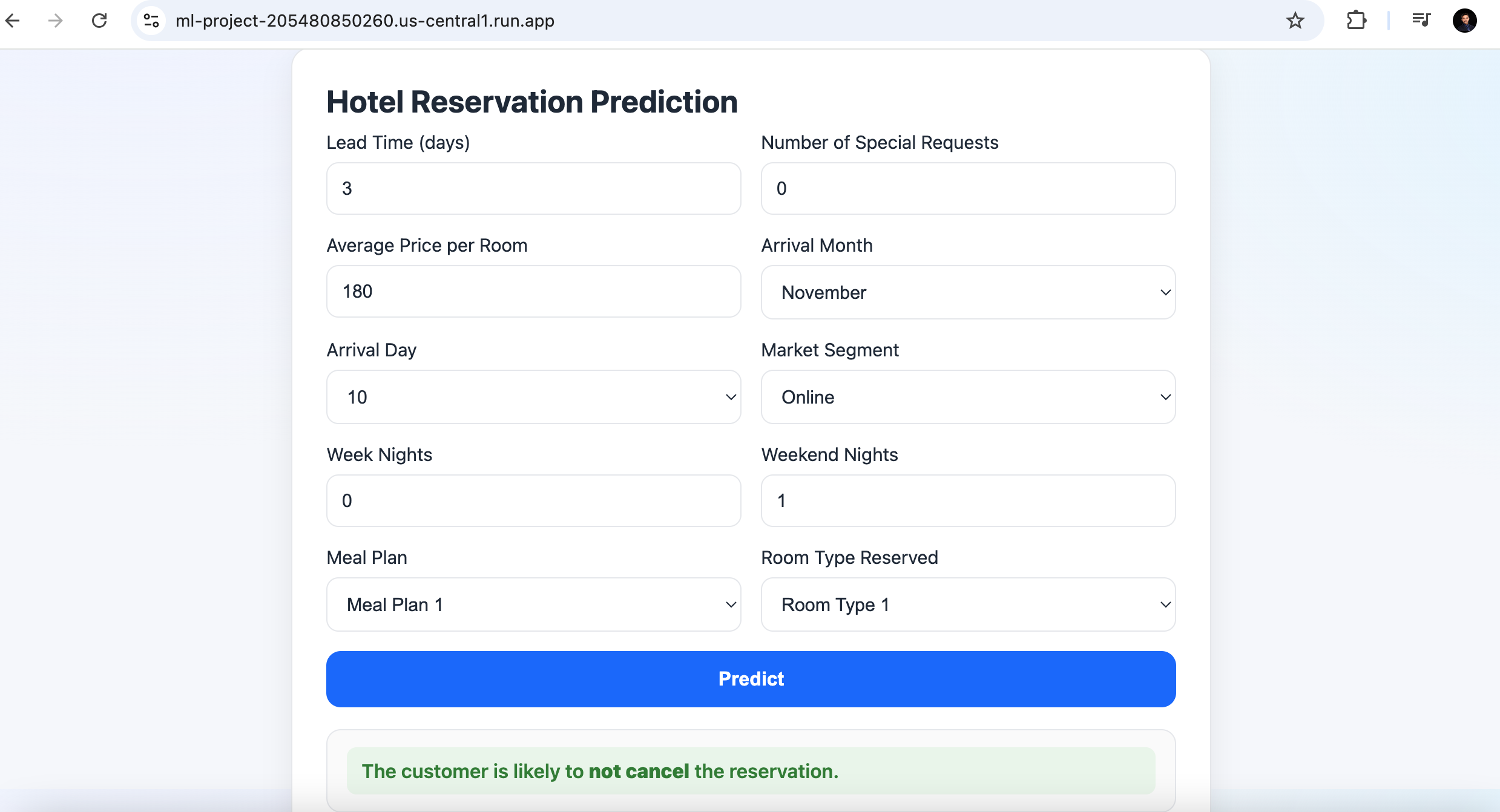
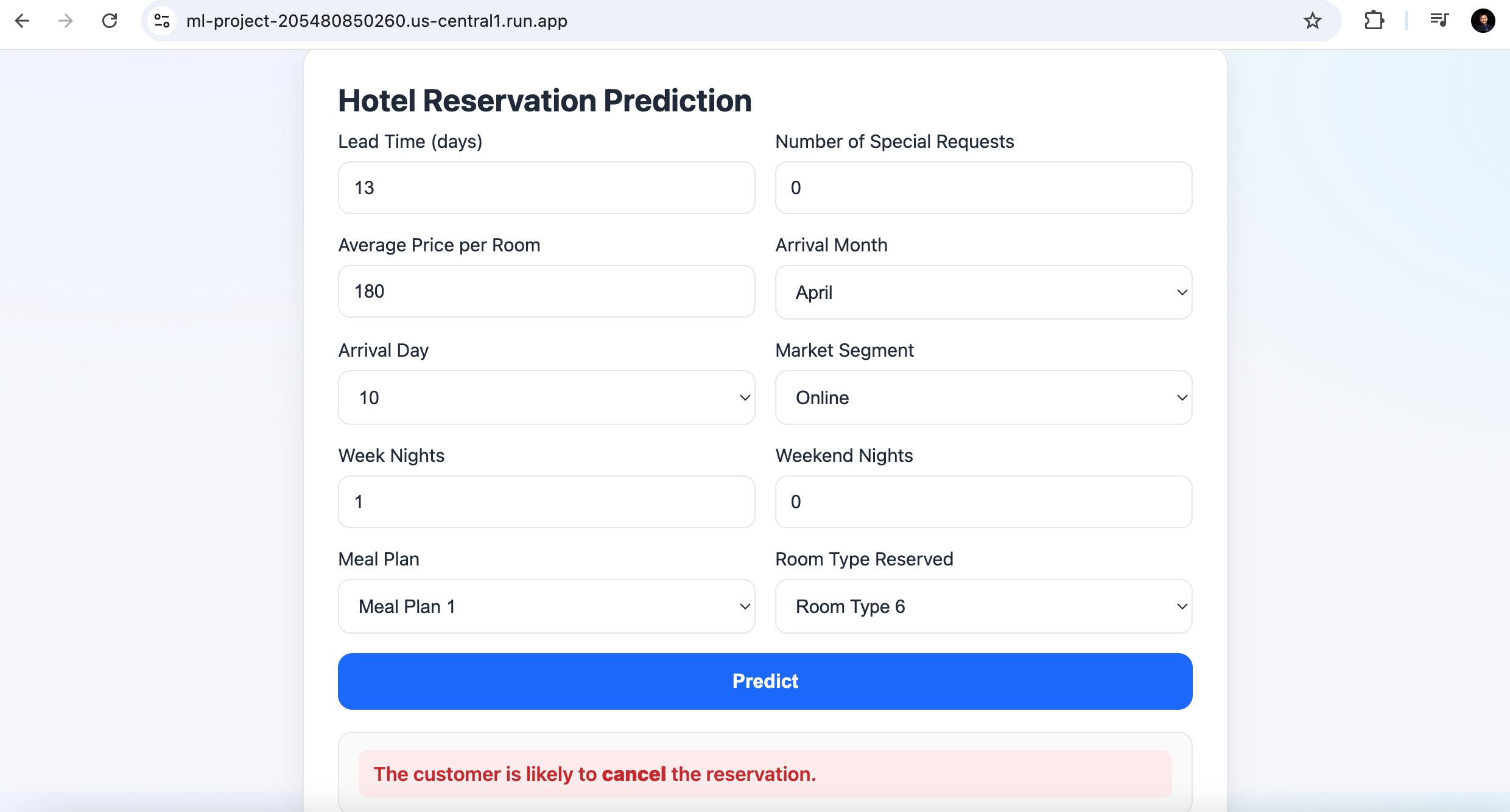
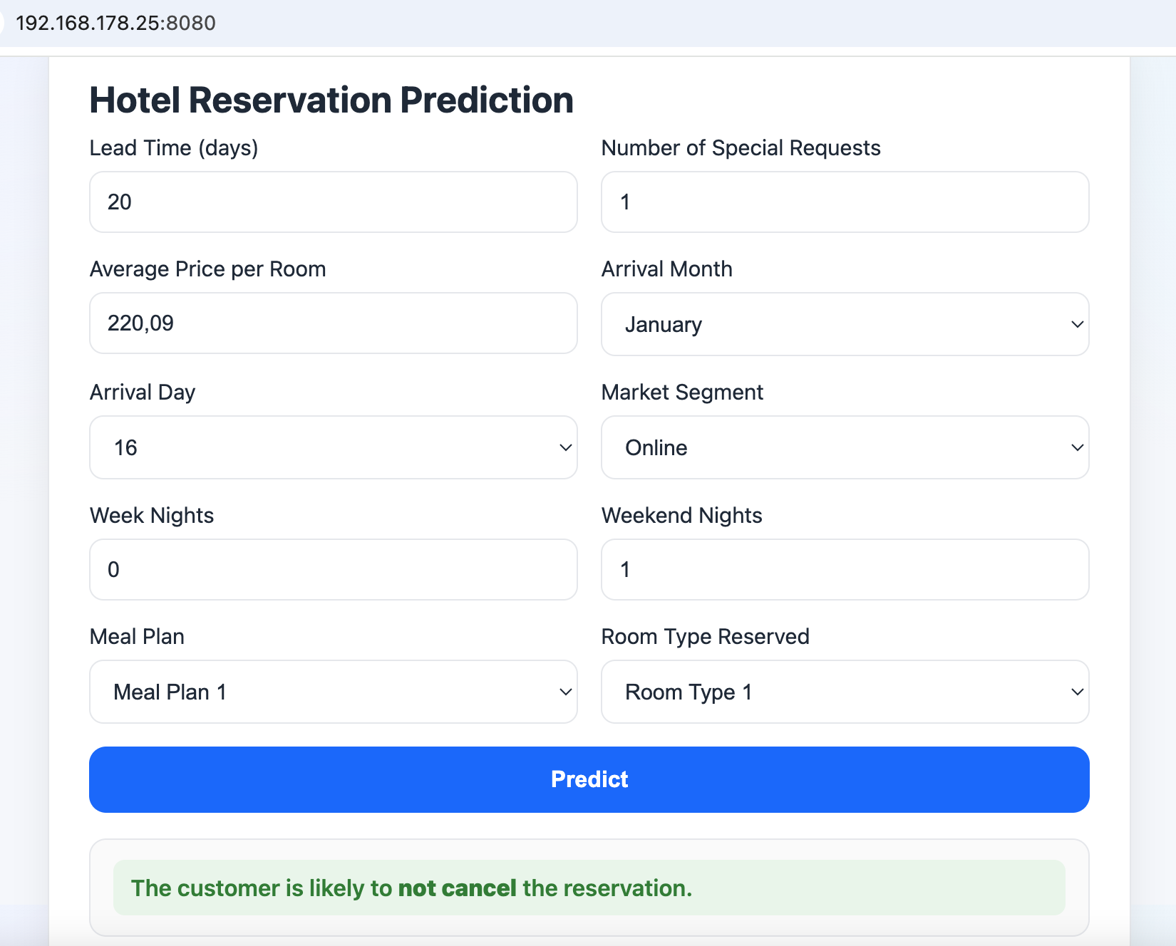
Cancellations hurt occupancy forecasts and revenue. If we can predict, at booking time, whether a reservation is likely to be canceled, the hotel can adjust inventory, pricing, and outreach more intelligently. This project takes a real-world dataset of hotel reservations and turns it into a production web app that scores bookings in real time.

High-level outcome: In offline experiments, a Random Forest delivered the best accuracy but produced a ~168 MB artifact—too heavy for fast, low-cost serving. I deployed LightGBM instead: nearly identical accuracy with a much smaller model footprint, which lowers container size, startup latency, and Cloud Run costs.

View the source on GitHub

The experimentation notebook: from EDA to model choice

I started in a Jupyter notebook (experimentation.ipynb) to quickly iterate.

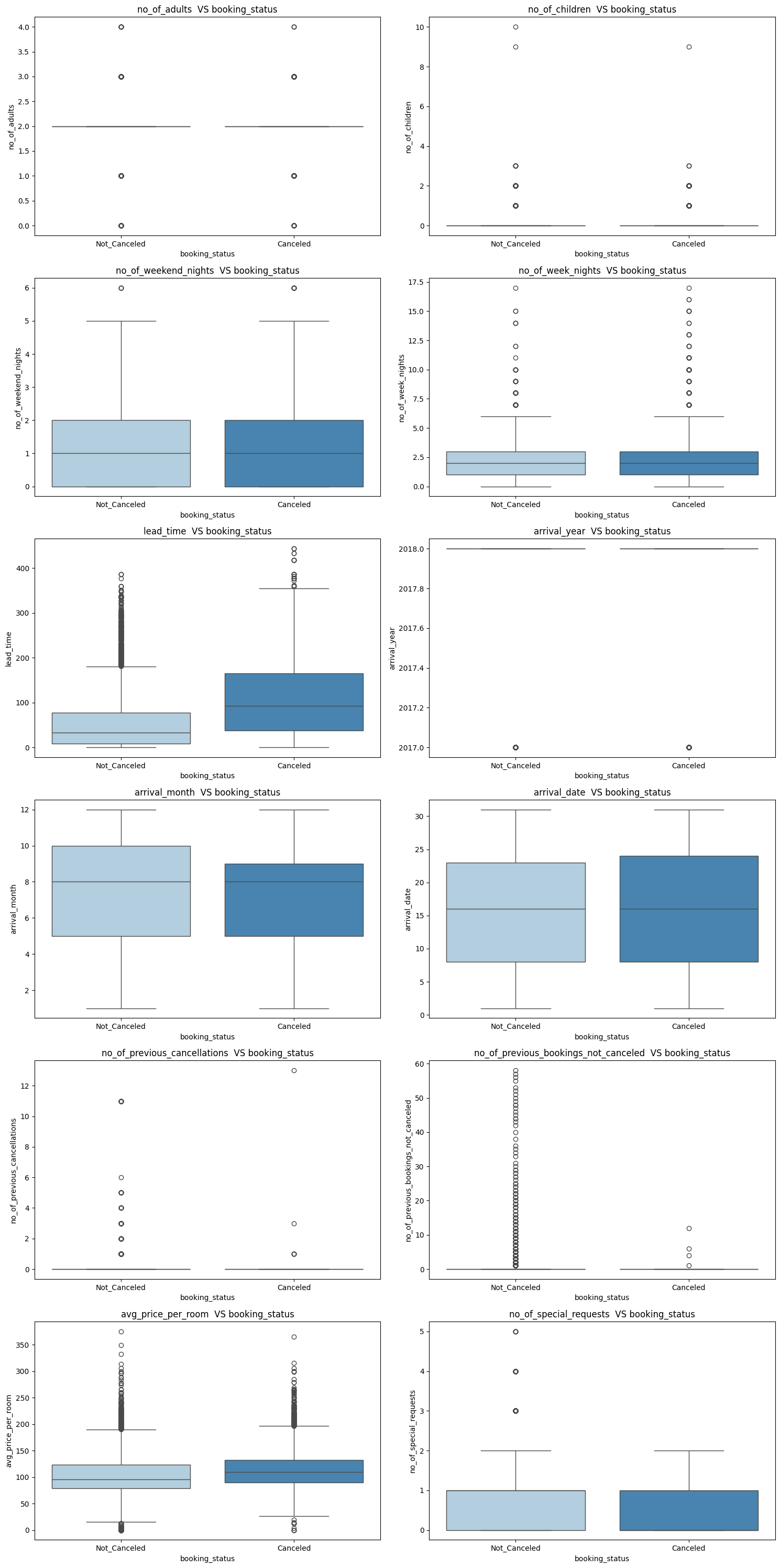
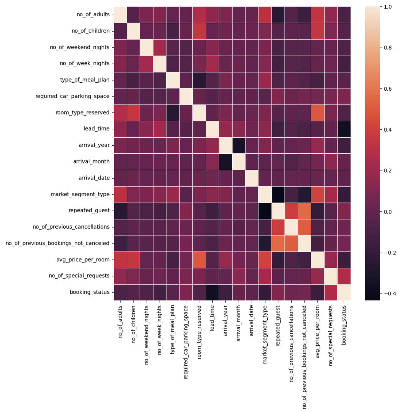
EDA highlights

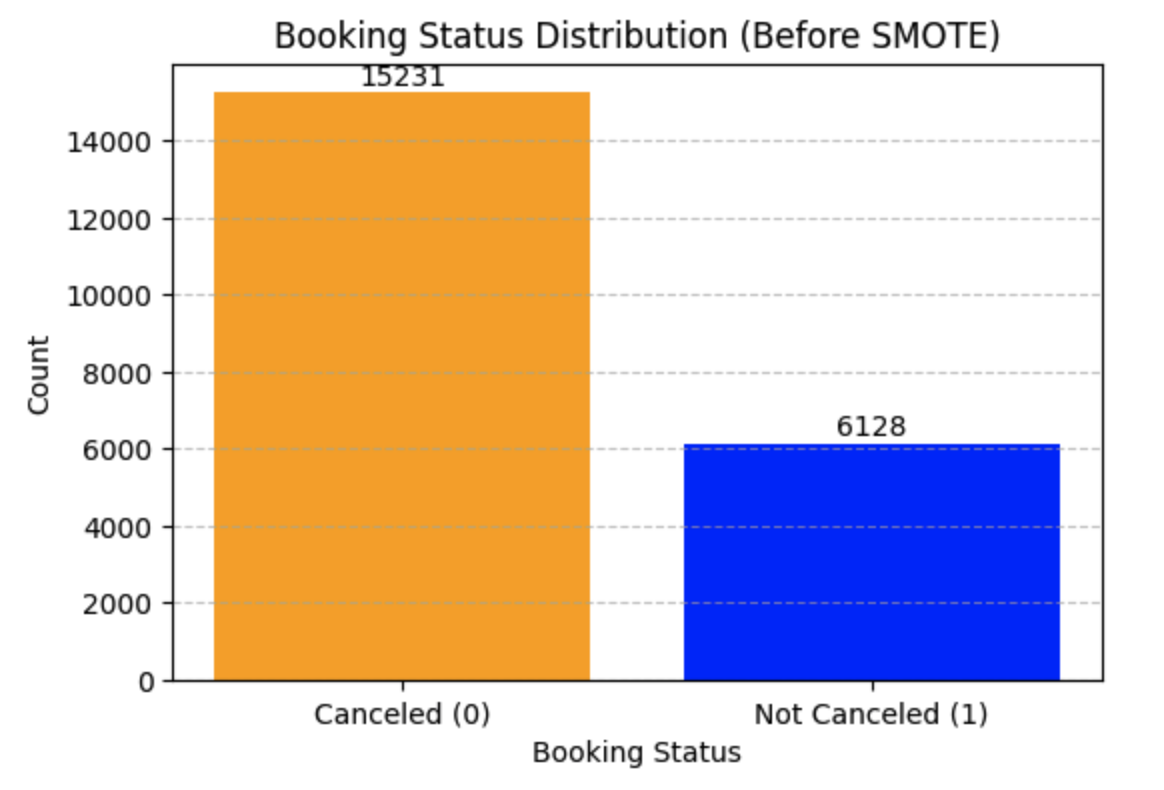
• Target balance: Checked cancellation distribution to understand class imbalance.
• Data cleaning: Removed duplicate rows; dropped Booking_ID and Unnamed: 0.
• Categoricals & numerics: Reviewed distributions for features like market_segment_type, type_of_meal_plan, room_type_reserved; examined skew for lead_time and avg_price_per_room.
• Leakage scan: Ensured no post-booking signals leak into training.

Feature engineering & preprocessing (prototyped)

• Label encoding for categorical columns (kept mappings).
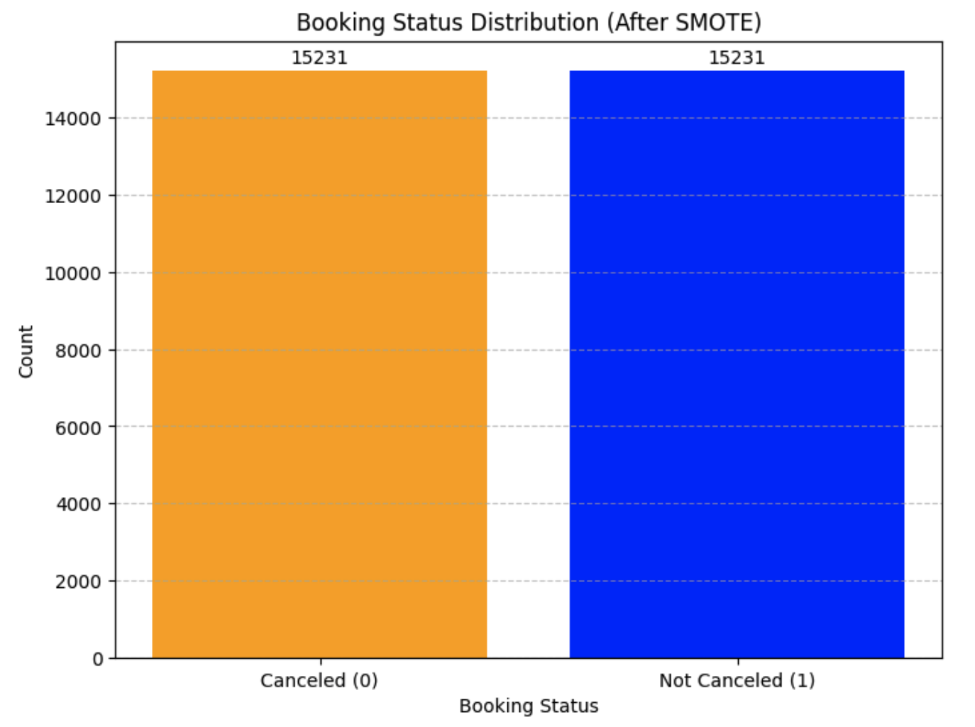
• Skewness handling: log1p for skewed numeric columns above a threshold.
• SMOTE: Balanced the training set when needed.
• Feature selection: Trained a quick Random Forest to get importances, then selected top-K features (configurable).

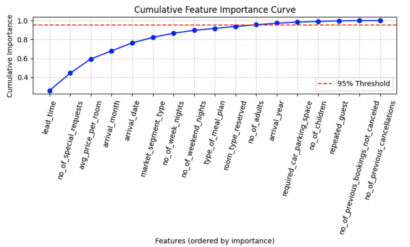
• Lead time is the strongest predictor — guests booking far in advance show higher cancellation likelihood.
• Customer engagement indicators like no_of_special_requests significantly reduce cancellations.
• Pricing (avg_price_per_room) plays a major role, with rate changes influencing booking behavior.
• Seasonality (arrival_month, arrival_date) impacts cancellation trends, reflecting peak/off-peak periods.

Model trials

• Baselines: Logistic Regression, Random Forest, XGBoost, LightGBM.
• Metrics: Accuracy (primary), plus Precision/Recall/F1.
• Results: Random Forest topped accuracy but yielded a ~168 MB model. LightGBM was nearly as accurate but much smaller; this trade-off drove the deployment decision.

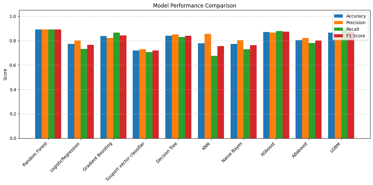
• Random Forest achieved the highest overall performance with Accuracy, Precision, Recall, and F1 all at ~0.893, indicating a well-balanced and reliable model.
• XGBoost and LightGBM followed closely, with slightly lower accuracy but strong recall, making them good choices if capturing more cancellations is a priority.
• Gradient Boosting offered a good recall boost (0.865) but slightly lower accuracy than Random Forest.
• Logistic Regression and Naive Bayes performed moderately, but their recall lagged, meaning they might miss more cancellations.
• Support Vector Classifier and KNN had the weakest overall balance, suggesting they may not be optimal for this dataset.

Recommendation: If you prioritize balanced performance, go with Random Forest. If you prioritize smaller model size and higher recall (catching cancellations even at slight accuracy cost), consider LightGBM or XGBoost.

Hardening the code: turning notebook steps into modules

After validating the approach in the notebook, I ported the logic into a clean, testable package with config-driven behavior and consistent logging.

Key modules

• src/logger.py – Centralized logging (file + console), sensible formats/levels.
• src/custom_exception.py – Exceptions with file/line context and original error chaining.
• utils/utility_functions.py – Helpers to read YAML config and load CSV robustly.

• src/data_ingestion.py

  • Downloads the raw CSV from GCS (bucket + blob from config/config.yaml) using Application Default Credentials.
  • Splits train/test by ratio; writes to data/raw/….

• src/data_preprocessing.py

  • Drops unneeded columns, deduplicates.
  • Label-encodes configured categoricals; logs mappings for traceability.
  • Applies log1p to skewed numerics above threshold.
  • Balances with SMOTE (train set).
  • Performs feature selection with RF importances; keeps top-K + target.
  • Saves processed train/test to constants: PROCESSED_TRAIN_DATA_PATH, PROCESSED_TEST_DATA_PATH.

• src/model_training.py

  • Loads processed data, splits features/target.
  • LightGBM tuned via RandomizedSearchCV (configurable params).
  • Computes Accuracy/Precision/Recall/F1 (binary-safe with zero_division=0).
  • Saves the best model (joblib) to MODEL_OUTPUT_PATH.
  • Logs datasets, params, and metrics to MLflow.

• pipeline/training_pipeline.py

  • Orchestrates: Ingestion → Preprocessing → Training
  • One function call run_pipeline() runs the end-to-end process with clear stage logs and robust error handling.

Serving layer: a simple Flask app

The app is intentionally straightforward for portability and clarity.

• application.py loads the trained joblib model from MODEL_OUTPUT_PATH.

• templates/index.html + static/style.css provide a small form to enter the 10 features used in training:

  • lead_time, no_of_special_request, avg_price_per_room, arrival_month, arrival_date, market_segment_type, no_of_week_nights, no_of_weekend_nights, type_of_meal_plan, room_type_reserved
• On POST, the app constructs a feature vector in the exact order used during training and returns a cancellation prediction (cancel / not cancel).

CI/CD & cloud deployment on GCP (Jenkins + Docker + Cloud Run)

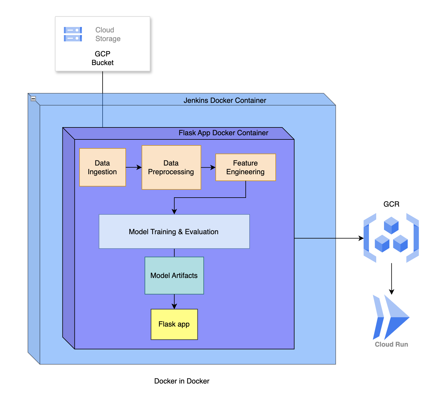
Why not train during docker build?

Running the training step inside docker build forces credentials into an image layer and complicates google-auth defaults. It also made builds flaky. I moved training out of the Dockerfile and into the Jenkins pipeline (with properly scoped credentials), then baked the resulting model artifact into the runtime image.

Dockerfile (runtime-only image)

• Based on python:slim
• Installs system deps (e.g., libgomp1 for LightGBM)
• Copies the repo and installs the package
• Does not train—just runs application.py on port 8080

Jenkins pipeline (Option A: train first, then build)

Stages:

1. Clone repo
2. Create venv & install: pip install -e .

3. Train model (with ADC):

   • Jenkins injects the GCP service account file as a credential (withCredentials(file: ...)).
   • Runs pipeline/training_pipeline.py which downloads data from GCS, preprocesses, and trains LightGBM.
   • The model is saved under the repo at MODEL_OUTPUT_PATH so it gets included by COPY . . later.

4. Build & push image:

   • Tags with both commit SHA and latest
   • Pushes to GCR (gcr.io/<project>/ml-project)

5. Deploy to Cloud Run:

   • gcloud run deploy ml-project --image gcr.io/<project>/ml-project:<sha> --region us-central1 --platform managed --port 8080 --allow-unauthenticated

Secrets & configuration

• ADC only during training in Jenkins; never copied into the image.
• The app reads the model from MODEL_OUTPUT_PATH at runtime; no cloud credentials are required for serving.
• A .dockerignore keeps images lean (venv/, .git/, caches, local artifacts).

Results & trade-offs

• Best offline model: Random Forest (highest accuracy), but ~168 MB.
• Deployed model: LightGBM (near-parity accuracy), significantly smaller binary.
• Operational benefits: Faster container pulls, quicker cold starts on Cloud Run, and lower memory footprint → lower cost and better UX.

What I’d improve next

• Persist and load label mappings so the UI can submit human-readable values and the server maps them to model codes robustly.
• Add AUC/PR-AUC for a fuller performance picture.
• MLflow model registry + staged promotions (Staging → Production).
• Monitoring & retraining triggers (Cloud Run logs + periodic data drift checks).
• Traffic-split canaries on Cloud Run for safe rollouts.

Run it yourself (dev)

# train locally (needs GCP ADC only for data ingestion)
python -m venv .venv && source .venv/bin/activate
pip install -e .
export GOOGLE_APPLICATION_CREDENTIALS=/path/to/sa.json
python pipeline/training_pipeline.py

# serve locally
python application.py  # http://localhost:8080

Production is handled by Jenkins: train → build → push → deploy.

Closing

This project shows the full lifecycle: notebook exploration → modular pipeline → CI/CD → cloud deployment. The key engineering decision was choosing a model that balances accuracy with deployability. LightGBM gave us similar predictive performance with a fraction of the size, which paid off immediately in speed and cost once the service went live.